3 - The Swarm-Verse

Marina Papadopoulou

After having analyzed our data, we can examine the intra- and inter-specific variation present across datasets through dimensionality reduction techniques (create ‘swarm spaces’).

3.1 Load data

Load the metrics of collective motion calculated previously. Include the events you want to compare in a swarm space.

library(swaRmverse)

# load pacakge data for many species
data("multi_species_metrics")

## A] Create the swarm space for this data only:
all_data <- multi_species_metrics

## B] Or bind with new data if continuing from step2
data("new_species_metrics") ## loads the output of step 2

new_species_tobind <- new_species_metrics[,!colnames(new_species_metrics) %in% c('event_dur', 'N', 'set', 'start_time')] # remove columns not needed for the swarm space
all_data <- rbind(multi_species_metrics, new_species_tobind)

## C] Or to use just the new data (overwrites previous command, comment out to compare with the other species):
all_data <- new_species_metrics

3.2 Build swarm space

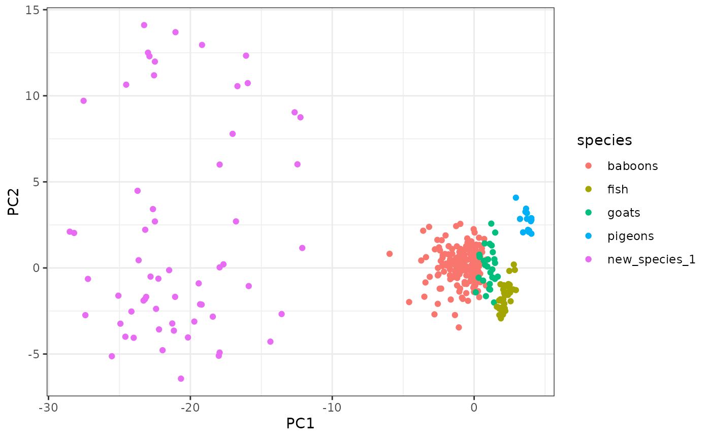
Create new swarm space with PCA analysis:

new_pca <- swarm_space(metrics_data = all_data,
                       space_type = "pca"
                       )

ggplot2::ggplot(new_pca$swarm_space,
                 ggplot2::aes(x = PC1, y = PC2, color = species)
                ) +
                ggplot2::geom_point() +
                ggplot2::theme_bw()

Check what each principal component represents and get the info of each event:

pca_info <- new_pca$pca$rotation[, new_pca$pca$sdev > 1]
print(pca_info)

##                          PC1         PC2          PC3         PC4
## mean_mean_nnd   -0.120557087 -0.47823789 -0.198936000  0.51970748
## mean_sd_nnd      0.006773648 -0.19922584 -0.693308303  0.22378356
## sd_mean_nnd      0.096140524 -0.33849821  0.445329654 -0.12538046
## mean_pol         0.169686225 -0.42069450 -0.035516371 -0.32822763
## sd_pol           0.551102219  0.02143889 -0.114126771 -0.07014666
## cv_speed         0.535969436 -0.10620905  0.006046155 -0.00581108
## mean_sd_front    0.168816754  0.01838288  0.267740886  0.61225187
## mean_mean_bangl -0.048978601 -0.53599416  0.352446821  0.09556011
## mean_shape       0.154168969  0.37491589  0.242066756  0.40886134
## sd_shape         0.549309319  0.01015417 -0.112278306  0.01629187

ref_data <- new_pca$ref
head(ref_data)

##   event N             set          start_time event_dur       species
## 1     1 8 2020-02-01_ctx1 2020-02-01 12:00:21      1.28 new_species_1
## 2     2 8 2020-02-01_ctx1 2020-02-01 12:00:23      1.12 new_species_1
## 3     3 7 2020-02-01_ctx1 2020-02-01 12:00:25      1.08 new_species_1
## 4     4 8 2020-02-01_ctx1 2020-02-01 12:00:26      0.04 new_species_1
## 5     5 8 2020-02-01_ctx1 2020-02-01 12:00:27      0.32 new_species_1
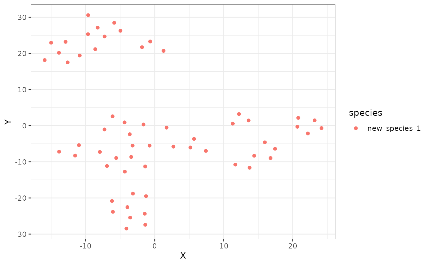
## 6     6 7 2020-02-01_ctx1 2020-02-01 12:00:28      7.80 new_species_1

Or create a new swarm space with tSNE to better study the local structure of the data:

new_tsne <- swarm_space(metrics_data = all_data,
                              space_type = "tsne",
                              tsne_rand_seed = 2023,
                              tsne_perplexity = 10
                              )

print("t-SNE was run with the following parameters:")

## [1] "t-SNE was run with the following parameters:"

print(new_tsne$tsne_setup)

##          prop  vals
## 1  perplexity    10
## 2 random_seed  2023
## 3    max_iter 10000

ggplot2::ggplot(new_tsne$swarm_space, ggplot2::aes(x = X, y = Y, color = species)) +
  ggplot2::geom_point() +
  ggplot2::theme_bw()

3.3 Expand existing swarm space

Starting from previously generated PCA swarm space, add new data:

data("multi_species_pca")
data("multi_species_pca_data")

new_pca_data <- expand_pca_swarm_space(metrics_data = new_species_metrics,
                                       pca_space = multi_species_pca)

expanded_pca <- rbind(multi_species_pca_data, 
                      new_pca_data)

ggplot2::ggplot(expanded_pca,
                ggplot2::aes(x = PC1, y = PC2, color = species)) +
   ggplot2::geom_point() +
   ggplot2::theme_bw()

3.4 Your own swarm space

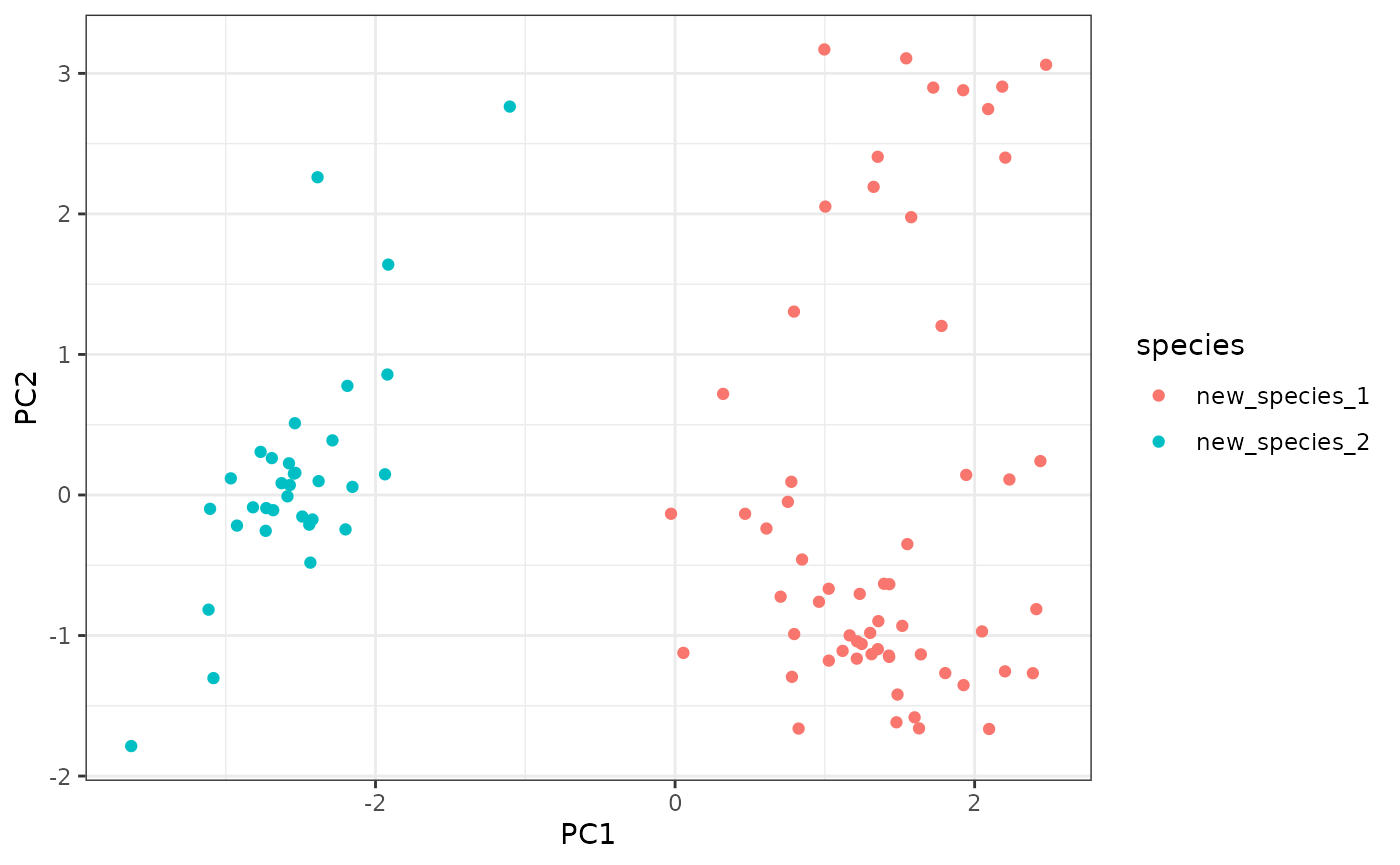
To compare several new datasets, one should run the analysis until the end of step 2 for each one of them. Then simply bind the result datasets together and run the swarm spaces as above:

data("new_species_metrics") ## loads the output of step 2

## Use another dataset:
data_df <- get(data("tracks", package = "trackdf"))
data_df$set <- as.Date(data_df$t)

another_species <- col_motion_metrics_from_raw(data_df,
                                mov_av_time_window = 10,
                                step2time = 1,
                                geo = TRUE,
                                verbose = FALSE,
                                speed_lim = 0,
                                pol_lim = 0.3,
                                parallelize_all = FALSE
                                )

another_species$species <- "new_species_2"

## Bind all the datasets you want to compare here
all_data <- rbind(another_species, new_species_metrics)

new_pca <- swarm_space(metrics_data = all_data,
                       space_type = "pca"
                       )

ggplot2::ggplot(new_pca$swarm_space,
                ggplot2::aes(x = PC1, y = PC2, color = species)
                ) +
  ggplot2::geom_point() +
  ggplot2::theme_bw()